More About the Math:
The Traveling Spike (Part 3)
Again, our equation for the axon voltage V (x; t) is:
\frac{1}{R} \frac{\partial^2 V(x,t)}{\partial x^2} = C
\frac{dV(x,t)}{dt} + \bar{g}_{Na} m(x,t)^3 h (V(x,t)-V_{Na}) -
\bar{g}_K n(x,t)^4 (V(x,t)-V_K) - g_L (V(x,t)-V_L)
The key challenge here is that this equation mixes changes in space x and
time t, that is, the rate of change of voltage in time depends on
the rate of change of voltage over space! This means that to figure out how a
solution evolves in time at one point x we need to keep track of,
hence evolve in time, the solution at all of the other spatial points.
Fortunately, there is a way to sidestep this difficulty. Remember what
we're looking for: a spike of fixed shape that travels down the axon
at a fixed
speed c. That is,
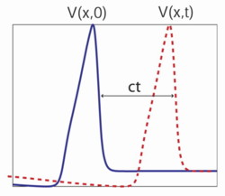
Note that the value of voltage at some point x at time t = 0 (V (x; 0)) is
the same as the voltage at the point x + ct at time t (V (x; t)).
That means that our solution V (x; t) is really just a function of a
(x - ct): V (x; t) = V (x - ct).
So, we have this crucial fact:
\frac{\partial^2
V(x,t)}{\partial x^2} = \frac{1}{c^2} \frac{\partial^2
V(x,t)}{\partial t^2} \;.
Therefore, our evolution equation is:
\frac{1}{Rc^2} \frac{\partial^2 V(x,t)}{\partial t^2} = C
\frac{dV(x,t)}{dt} + \bar{g}_{Na} m(x,t)^3 h (V(x,t)-V_{Na}) -
\bar{g}_K n(x,t)^4 (V(x,t)-V_K) - g_L (V(x,t)-V_L)
with only derivatives with respect to time (the same is true of equations
for m(x; t), h(x; t), and n(x; t)). So, we can solve
these equations using the methods we started out with for the space-independent
Hodgkin-Huxley equations. CLICK here to take this final step.