More About the Math:
Numerical Algorithms
Numerical solutions to differential equations
The Hodgkin-Huxley model is a set of four coupled nonlinear differential
equations. How does one solve these equations? To explain let
us abstract to a general nonlinear differential equation of one variable x.
\begin{eqnarray}
\frac{dx}{dt}=f(x)
\end{eqnarray}
Here f is some function of x (like x, x4,
or tan(x) for example) and dx/dt is the rate
of change of x with respect to time. Let us assume that
at an initial time t0 we know that x=x0 If f is
a linear equation, i.e f(x)=ax+b, then we can explicitly write
down the solution of x. Unfortunately, this is not true
in general for nonlinear equations, such as the Hodgkin-Huxley model. To
solve nonlinear differential equations it is typical to use an iterative
scheme to construct the solution from many sequential calculations.
Choose a discrete set of times t0<t1<t2<…<tN with ti+1 -
ti=\Deltat, we call \Deltat the
timestep. We consider a timestep that is much smaller than the timescale
over which the system evolves (\Deltat << 1 for a system
with timescale 1). This means that in the small time interval ti+1 – ti we
have that x(ti+1)-x(ti)=\Deltaxi is
also small.
Since \Deltat and \Deltaxi are
both small we can approximate their ratio with the derivative
\begin{eqnarray}
\frac{\Delta x_{i}}{\Delta t} \approx \frac{dx}{dt}(t_i)=f(x(t_i))
\end{eqnarray}
We can rearrange the equation, recalling that \Deltaxi=x(ti+1)
- x(ti), to give:
\begin{eqnarray}
x(t_{i+1})=x(t_i)+\Delta t f(x(t_i))
\end{eqnarray}
We can write x(ti) via the iterative scheme
\begin{eqnarray}
x(t_0)&=&x_0 \\
x(t_1)&=&x(t_0)+\Delta t f(x(t_0)) \\
x(t_2)&=&x(t_1)+\Delta t f(x(t_1)) \\
&\vdots& \\
x(t_N)&=&x(t_{N-1})+\Delta t f(x(t_{N-1}))
\end{eqnarray}
Given an initial condition x0 we can solve
for x(t) with
an accuracy that increases as \Deltat decreases. The price paid for increased
accuracy is that the number of iterations needed between t and t0 also
increases. With the computation speed of modern computers a small
\Deltat can be easily be chosen without seriously compromising speed. In
the 1950s Hodgkin and Huxley used a crank calculator, so they chose a balance
between speed and accuracy. Here is an example for a linear equation
where we compare the Euler approximation to the known solution.
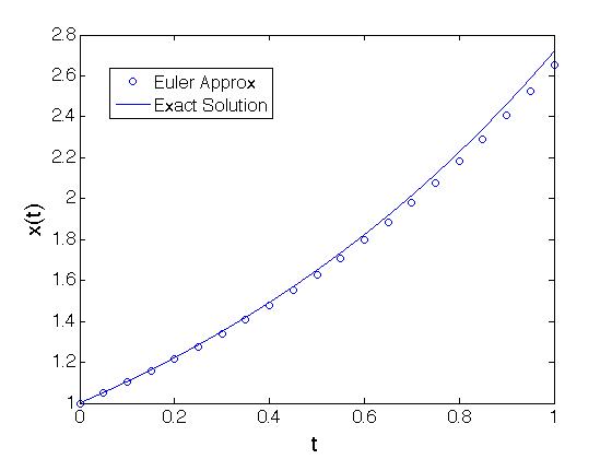
PLOT
The simple algorithm presented here explains the basic principals of the
more sophisticated numerical techniques used by Hodgkin and Huxley in the
1950s and are still in use today by many researchers in computational science.