Image Compression:

How Math Led to the JPEG2000 Standard

Basic JPEG

Introduction/History

In 1992, JPEG became an international standard for compressing digital still images. The acronym JPEG comes from the Joint Photographic Experts Group. JPEG was formed in the 1980's by members from the International Organization for Standardization (ISO) and the International Telecommunications Union (ITU). According to a 2000 article by Maryline Charrier et. al., over 80% of all images that are transmitted via the internet are stored using the JPEG standard. Despite the popularity of the standard, JPEG members quickly identified some issues with the format and also compiled a list of enhancements that should be included in the next generation of the format. In this section, we will describe a very basic JPEG algorithm, show how it works on an example, discuss the inversion process, and then identify issues and problems with the format.

Basic Algorithm


		A digital grayscale image. Fullsize version

The JPEG algorithm has many features that are not covered here. It is our intent to provide a very basic idea of how JPEG can be used to compress a digital still image. There are four basic steps in the algorithm - preprocess, transformation, quantization, encoding. We have already talked about Huffman coding and JPEG uses a more sophisticated version of Huffman coding to perform coding. We will not discuss the advanced coding methods used by JPEG here. Interested readers should consult a refence such as The Data Compression Book. For those readers interested in more details about the mathematics of transformation and quantization, please visit the subsections Discrete Cosine Transformation and Quantization.

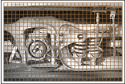
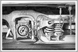
To explain the steps of the algorithm, we will use as a running example, the image above. The dimensions of the image 160 x 240 pixels.

Step 1 - Preprocessing

If we wish to compress a color image in the JPG format, the first step is to convert the red, green, blue color channels to YCbCr space. After that, everything we do for a grayscale image is done to the Y, Cb, and Cr channels.


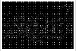
		Partitioning of the image into 8x8 blocks.

We next partition the image into blocks of size 8 x 8 pixels. Some more work is necessary if the dimensions of our image are not divisible by 8, but for the sake of presentation, we have chosen an image whose dimensions are 160 x 240 = 8*20 x 8*30. So this step creates 20 x 30 = 600 blocks.

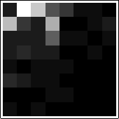
Notice that we have highlighted the pixels in block row 4, block column 28. We will use the elements of this matrix to illustrate the mathematics of transformation and quantization steps. An enlargement of this block appears below as well as the 64 pixels intensities that make up the block.



		Enlargement of the example block.

5	176	193	168	168	170	167	165
6	176	158	172	162	177	168	151
5	167	172	232	158	61	145	214
33	179	169	174	5	5	135	178
8	104	180	178	172	197	188	169
63	5	102	101	160	142	133	139
51	47	63	5	180	191	165	5
49	53	43	5	184	170	168	74

Pixel intensities of the block row 4, block column 28.

The last part of preprocessing the image is to subtract 127 from each pixel intensity in each block. This step centers the intensities about the value 0 and it is done to simple the mathematics of the transformation and quantization steps. For our running example block, here are the new values.

-122	49	66	41	41	43	40	38
-121	49	31	45	35	50	41	24
-122	40	45	105	31	-66	18	87
-94	52	42	47	-122	-122	8	51
-119	-23	53	51	45	70	61	42
-64	-122	-25	-26	33	15	6	12
-76	-80	-64	-122	53	64	38	-122
-78	-74	-84	-122	57	43	41	-53
Pixel intensity values less 127 in block row 4, block column 28.

Step 2 - Transformation

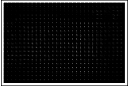
The preprocessing has done nothing that will make the coding portion of the algorithm more effective. The transformation step is the key to increasing the coder's effectiveness. The JPEG Image Compression Standard relies on the Discrete Cosine Transformation (DCT) to transform the image. The DCT is a product C = U B U^T where B is an 8 x 8 block from the preprocessed image and U is a special 8 x 8 matrix. More mathematical details about the DCT can be found in the subsection The Discrete Cosine Transformation. Loosely speaking, the DCT tends to push most of the high intensity information (larger values) in the 8 x 8 block to the upper left-hand of C with the remaining values in C taking on relatively small values. The DCT is applied to each 8 x 8 block. The image at left shows the DCT of our highlighted block while the image at right shows the DCT applied to each block of the preprocessed image.


		DCT of the example block.			DCT applied to each block. Fullsize version

As you can see, most of the intensities in the discrete cosine transformed image are quite small and at first glance, one might think that the Huffman coding scheme would work very well with the this image. But there are still some problems. Let's have a look at the values (rounded to three digits) of the DCT of our example block:

-27.500	-213.468	-149.608	-95.281	-103.750	-46.946	-58.717	27.226
168.229	51.611	-21.544	-239.520	-8.238	-24.495	-52.657	-96.621
-27.198	-31.236	-32.278	173.389	-51.141	-56.942	4.002	49.143
30.184	-43.070	-50.473	67.134	-14.115	11.139	71.010	18.039
19.500	8.460	33.589	-53.113	-36.750	2.918	-5.795	-18.387
-70.593	66.878	47.441	-32.614	-8.195	18.132	-22.994	6.631
12.078	-19.127	6.252	-55.157	85.586	-0.603	8.028	11.212
71.152	-38.373	-75.924	29.294	-16.451	-23.436	-4.213	15.624
DCT values in block row 4, block column 28.

The values in the matrix above have been rounded to 3 digits - in truth, most of the values are irrational numbers. Now most computers calculate the values (floating point numbers) to 16 digits (double precision) with the last digit being round-off error. Do you see the problem? The fact that the numbers are computed to 16 digits with round-off error in the last digit means that it is possible for a number to have two different representations! Thus, if we do nothing to modify this situation, the Huffman coding algorithm will not be effective. So the DCT does create a large number of near-zero values, but we need a quantization step to better prepare the data for coding.

Step 3 - Quantization

The next step in the JPEG algorithm is the quantization step. Here we will make decisions about values in the transformed image - elements near zero will converted to zero and other elements will be shrunk so that their values are closer to zero. All quantized values will then be rounded to integers.

Quantization makes the JPEG algorithm an example of lossy compression. The DCT step is completely invertible - that is, we applied the DCT to each block B by computing C = U B U^T. It turns out we can recover B by the computation B = U^T C U. When we "shrink" values, it is possible to recover them. However, converting small values to 0 and rounding all quantized values are not reversable steps. We forever lose the ability to recover the original image. We perform quantization in order to obtain integer values and to convert a large number of the values to 0. The Huffman coding algorithm will be much more effective with quantized data and the hope is that when we view the compressed image, we haven't given up too much resolution. For applications such as web browsing, the resolution lost in order to gain storage space/transfer speed is acceptable.

Let's have another look at the DCT of our original block and the values that comprise it:



		DCT of the example block.

-27.500	-213.468	-149.608	-95.281	-103.750	-46.946	-58.717	27.226
168.229	51.611	-21.544	-239.520	-8.238	-24.495	-52.657	-96.621
-27.198	-31.236	-32.278	173.389	-51.141	-56.942	4.002	49.143
30.184	-43.070	-50.473	67.134	-14.115	11.139	71.010	18.039
19.500	8.460	33.589	-53.113	-36.750	2.918	-5.795	-18.387
-70.593	66.878	47.441	-32.614	-8.195	18.132	-22.994	6.631
12.078	-19.127	6.252	-55.157	85.586	-0.603	8.028	11.212
71.152	-38.373	-75.924	29.294	-16.451	-23.436	-4.213	15.624

DCT values in block row 4, block column 28.

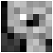
The mathematics of quantization is explained in the Quantization subsection. Here is the result of quantization applied to our example block. The image has been enhanced to facilitate viewing of the low intensities.



		Quantized DCT of the example block.

-2	-19	-15	-6	-4	-1	-1	0
14	4	-2	-13	0	0	-1	-2
-2	-2	-2	7	-1	-1	0	1
2	-3	-2	2	0	0	1	0
1	0	1	-1	-1	0	0	0
-3	2	1	-1	0	0	0	0
0	0	0	-1	1	0	0	0
1	0	-1	0	0	0	0	0

DCT values in block row 4, block column 28.

For comparison purposes, we have plotted the transformed image from above next to the quantized version of the transformed image. The second image has been enhanced to facilitate viewing.


		DCT applied to each block. Fullsize version			DCT and quantization applied to each block. Fullsize version

Step 4 - Encoding

The last step in the JPEG process is to encode the transformed and quantized image. The regular JPEG standard uses an advanced version of Huffman coding. We will use the basic Huffman coding algorithm described in the Compression in a Nutshell section. The original image has dimensions 160 x 240 so that 160*240*8 = 307,200 bits are needed to store it to disk. If we apply Huffman coding to the transformed and quantized version of the image, we need only 85,143 bits to store the image to disk. The compression rate is about 2.217bpp. This represents a savings of over 70% of the original amount of bits needed to store the image!

Inverting the Process

The inversion process is quite straightforward. The first step is to decode the Huffman codes to obtain the quantized DCT of the image. In order to undo the shrinking process, elements in each 8x8 block are magnified by the appropriate amount (see the Quantization subsection for more details). At this point we have blocks C^' where the original DCT before quantization is C = U B U^T. We next invert the DCT by computing B^' = U^T C^'U for each block. The last step is to add 127 to each element in each block. The resulting matrix is an approximation to the original image.

The images below shows the original image at left and the JPEG compressed image at right. Recall that the image at right requires over 70% less storage space than that of the original image!


		A digital grayscale image. Fullsize version			The compressed grayscale image. Fullsize version

Finally, we compare our example of block row 4, block column 28 with the compressed version of the block.



		Enlargement of the block.

5	176	193	168	168	170	167	165
6	176	158	172	162	177	168	151
5	167	172	232	158	61	145	214
33	179	169	174	5	5	135	178
8	104	180	178	172	197	188	169
63	5	102	101	160	142	133	139
51	47	63	5	180	191	165	5
49	53	43	5	184	170	168	74

Pixel intensities of the block.



		Enlargement of the compressed block.

0	172	198	190	149	159	149	179
17	166	131	175	168	195	192	140
12	167	177	255	140	39	123	203
22	178	170	145	1	28	146	187
11	103	183	190	160	207	189	155
60	9	80	103	157	144	115	156
60	48	67	11	176	196	139	19
49	58	47	0	190	168	176	60

Pixel intensities of the compressed block.

Issues and Problems

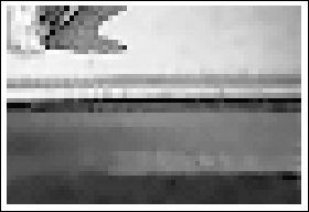
The JPEG Image Compression Standard is a very effective method for compressing digital images, but it does suffer from some problems. One problem is the decoupling that occurs before we apply the DCT - partitioning the image into 8x8 blocks results in the compressed image sometimes appearing "blocky". In the images below, we have zoomed in on the upper right hand corners of the original image and the compressed image. You can see the block artifacts in the compressed image.


		Upper right hand corner of original image. Fullsize version			Upper right hand corner of compressed image. Fullsize version

The quantization step makes the JPEG Image Compression Standard an example of lossy compression. For some applications, such as web browsing, the loss of resolution is acceptable. For other applications, such as high resolution photographs for magazine advertisements, the loss of resolution is unacceptable.

As you will see in the Features/Enhancements subsection of the JPEG2000 section, researchers have found a better transformation and quantization methods to address the problems encountered by the JPEG standard.